3.2.8. IP Inversion Input File

The inverse problem is solved using the executable program ipoctree_inv.exe. The lines of input file are as follows:

Line #	Description	Description
1	OcTree Mesh	path to octree mesh file
2	Observations File	path to observations file
3	Initial/FWD Model	initial/forward model
4	Reference Model	reference model
5	Background Conductivity Model	reference model
6	Active Topography Cells	topography
7	Active Model Cells	active model cells
8	Global Cell Weights	global cell weights
9	Global Face Weights	global face weights
10	Cell Weights in Smallness Term	additional cell weights in smallness term
11	beta_max beta_min beta_factor	cooling schedule for beta parameter
12	alpha_s alpha_x alpha_y alpha_z	weighting constants for smallness and smoothness constraints
13	Chi Factor	stopping criteria for inversion
14	tol_nl mindm iter_per_beta	set the number of Gauss-Newton iteration for each beta value
15	tol_ipcg max_iter_ipcg	set the tolerance and number of iterations for Gauss-Newton solve
16	Reference Model Update	reference model
17	Hard Constraints	use SMOOTH_MOD or SMOOTH_MOD_DIFF
18	Bounds	upper and lower bounds for recovered model

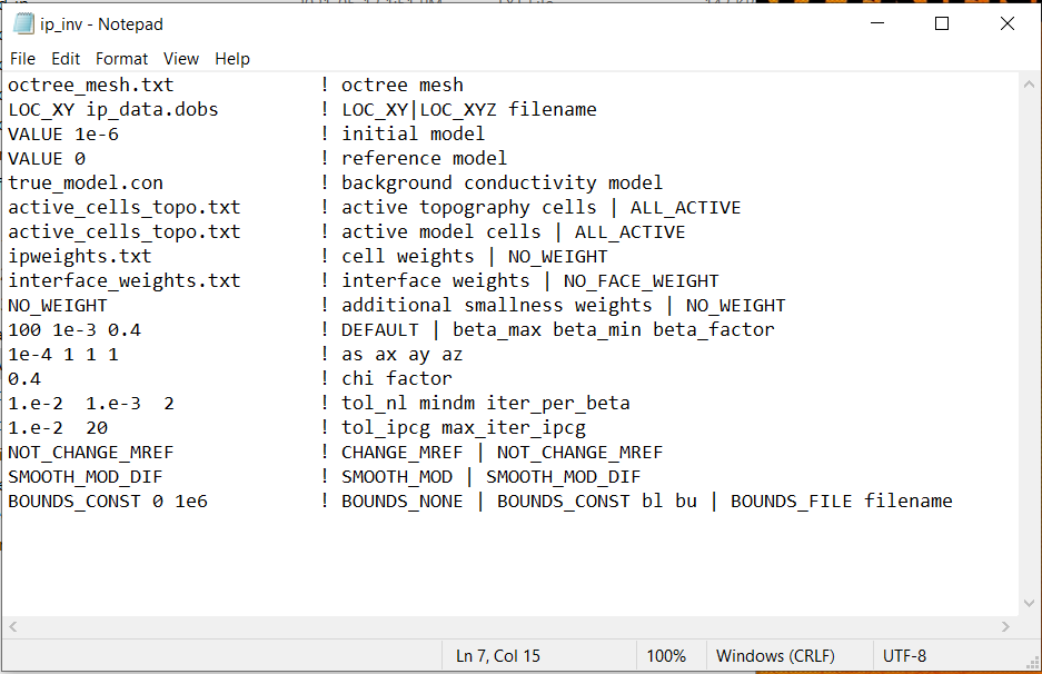
Fig. 3.9 Example input file for the inversion program (Download ).

3.2.8.1. Line Descriptions

• OcTree Mesh: file path to the OcTree mesh file

• Observation File: On this line, we enter a flag LOC_XY or LOC_XYZ, followed by the file path to the observations file. The flag tells the program whether the electrodes are only on the surface or whether there are borehole measurements.

  • LOC_XY filepath: The electrodes are all projected to the discrete surface topograpy. If Active Topography Cells line is set to ALL_ACTIVE, the electrodes are placed on the top of the mesh.

  • LOC_XYZ filepath: Electrodes remain at the exact xyz locations in the observations file. Necessary for borehole data.

• Initial Model: On this line we specify the starting model for the inversion. On this line, there are 2 possible options:

  • Enter the path to a chargeability model

  • If a homogeneous chargeability value is being used, enter “VALUE” followed by a space and a numerical value; example “VALUE 1e-5”. Do not set the starting model to all 0s or the algorithm will not be able to find a step direction on the first iteration. In this case, you may set the starting modeling to some small value (1e-5)

• Reference Model: The user may supply the file path to a reference model. On this line, there are 2 possible options:

  • Enter the path to a chargeability model

  • If a homogeneous chargeability value is being used, enter “VALUE” followed by a space and a numerical value; example “VALUE 1e-5”. Unlike the starting model, you can set the reference model to be zero.

• Background Conductivity Model: file path to a conductivity model.

• Active Topography Cells: Here, the user can choose to specify the cells which lie below the surface topography. To do this, the user may supply the file path to an active cells model file or type “ALL_ACTIVE”. The active cells model has values 1 for cells lying below the surface topography and values 0 for cells lying above.

• Active Model Cells: Here, the user can choose to specify the model cells which are active during the inversion. To do this, the user may supply the file path to an active cells model file or type “ALL_ACTIVE”. The active cells model has values 1 for cells lying below the surface topography and values 0 for cells lying above. Values for inactive cells are provided by the background conductivity model.

• Global Cell Weights: Here, the user specifies cell weights that are applied in both the smallness and smoothness terms in the model objective function. The user can provide the file path to a cell weights file . If no cell weights are supplied, the user enters “NO_WEIGHT”.

• Global Face Weights: Here, the user specifies whether face weights are supplied. If so, the user provides the file path to a face weights file cell weights file. If no additional cell weights are supplied, the user enters “NO_FACE_WEIGHT”. The user may also enter “EKBLOM” for 1-norm approximation to recover sharper edges.

• Cell Weights in Smallness Terms: Here, the user can specify cell weights that are ONLY applied to the smallness term in the model objective function; e.g. they are not used in the smoothness. The user can provide the file path to a cell weights file . For no additional weighting, the user enters the flag “NO_WEIGHT”.

• beta_max beta_min beta_factor: Here, the user specifies protocols for the trade-off parameter (beta). beta_max is the initial value of beta, beta_min is the minimum allowable beta the program can use before quitting and beta_factor defines the factor by which beta is decreased at each iteration; example “1E4 10 0.2”. The user may also enter “DEFAULT” if they wish to have beta calculated automatically.

• alpha_s alpha_x alpha_y alpha_z: Alpha parameters . Here, the user specifies the relative weighting between the smallness and smoothness component penalties on the recovered models.

• Chi Factor: The chi factor defines the target misfit for the inversion. A chi factor of 1 means the target misfit is equal to the total number of data observations.

• tol_nl mindm iter_per_beta: Here, the user specifies the number of Newton iterations. tol_nl is the Newton iteration tolerance (how close the gradient is to zero), mindm is the minimum model perturbation \(\delta m\) allowed and iter_per_beta is the number of iterations per beta value.

• tol_ipcg max_iter_ipcg: Here, the user specifies solver parameters. tol_ipcg defines how well the iterative solver does when solving for \(\delta m\) and max_iter_ipcg is the maximum iterations of incomplete-preconditioned-conjugate gradient.

• Reference Model Update: Here, the user specifies whether the reference model is updated at each inversion step result. If so, enter “CHANGE_MREF”. If not, enter “NOT_CHANGE_MREF”.

• Hard Constraints: SMOOTH_MOD runs the inversion without implementing a reference model (essential \(m_{ref}=0\)). “SMOOTH_MOD_DIF” constrains the inversion in the smallness and smoothness terms using a reference model.

• Bounds: Bound constraints on the recovered model. There are 3 options:

  • Enter the flag “BOUNDS_NONE” if the inversion is unbounded, or if there is no a-prior information about the subsurface model

  • Enter “BOUNDS_CONST” and enter the values of the minimum and maximum model conductivity; example “BOUNDS_CONST 1E-6 0.1”

  • Enter “BOUNDS_FILE” followed by the path to a bounds file