3.3.3. Observations File

Observations files can be used invert data with dcoctree_inv.exe or ipoctree_inv.exe. They can also be used to predict DC and/or IP data with dcipoctree_fwd.exe. Regardless of whether you are inverting DC or IP data, the format is the same. However, the definition of the data and uncertainties will be different.

The general format for observed data files is shown below.

Note

The [ ] brackets are used for columns are not always required. For surface formatted files, the Z values are omitted. For general formatted files, the Z values must be included.


[IPTYPE=1,2]

\(\;\;\;X_A(1) \;\;\;\;\;\;\;\; Y_A(1) \;\;\;\;\;\;\;\, [Z_A(1)] \;\;\;\;\;\;\; X_B(1) \;\;\;\;\;\;\; Y_B(1) \;\;\;\;\;\;\;\; [Z_B(1)] \;\;\;\;\;\;\;\;\;\; N\)
\(\;X_M(1,1) \;\;\; Y_M(1,1) \;\;\;\, [Z_M(1,1)] \;\;\;\, X_N(1,1) \;\;\;\, Y_N(1,1) \;\;\;\, [Z_N(1,1)] \;\;\; data(1,1) \;\;\; unc(1,3)\)
\(\;X_M(1,2) \;\;\; Y_M(1,2) \;\;\;\, [Z_M(1,2)] \;\;\;\, X_N(1,2) \;\;\;\, Y_N(1,2) \;\;\;\, [Z_N(1,2)] \;\;\; data(1,2) \;\;\; unc(1,3)\)
\(\;X_M(1,3) \;\;\; Y_M(1,3) \;\;\;\, [Z_M(1,3)] \;\;\;\, X_N(1,3) \;\;\;\, Y_N(1,3) \;\;\;\, [Z_N(1,3)] \;\;\; data(1,3) \;\;\; unc(1,3)\)
\(\;\;\;\;\;\;\;\;\;\vdots\;\;\;\;\;\;\;\;\;\;\;\;\;\;\vdots\;\;\;\;\;\;\;\;\;\;\;\;\;\;\;\;\;\vdots\;\;\;\;\;\;\;\;\;\;\;\;\;\;\;\;\;\;\vdots\;\;\;\;\;\;\;\;\;\;\;\;\;\;\;\;\vdots\;\;\;\;\;\;\;\;\;\;\;\;\;\;\;\;\vdots\;\;\;\;\;\;\;\;\;\;\;\;\;\;\;\;\;\;\vdots\;\;\;\;\;\;\;\;\;\;\;\;\;\;\;\;\;\,\vdots\)
\(X_M(1,N) \;\; Y_M(1,N) \;\; [Z_M(1,N)] \;\; X_N(1,N) \;\; Y_N(1,N) \;\; [Z_N(1,N)] \;\; data(1,N) \;\; unc(1,N)\)

\(\;\;\;X_A(2) \;\;\;\;\;\;\;\; Y_A(2) \;\;\;\;\;\;\;\, [Z_A(2)] \;\;\;\;\;\;\; X_B(2) \;\;\;\;\;\;\; Y_B(2) \;\;\;\;\;\;\;\; [Z_B(2)] \;\;\;\;\;\;\;\;\;\; N\)
\(\;X_M(2,1) \;\;\; Y_M(2,1) \;\;\;\, [Z_M(2,1)] \;\;\;\, X_N(2,1) \;\;\;\, Y_N(2,1) \;\;\;\, [Z_N(2,1)] \;\;\; data(2,1) \;\;\; unc(2,3)\)
\(\;X_M(2,2) \;\;\; Y_M(2,2) \;\;\;\, [Z_M(2,2)] \;\;\;\, X_N(2,2) \;\;\;\, Y_N(2,2) \;\;\;\, [Z_N(2,2)] \;\;\; data(2,2) \;\;\; unc(2,3)\)
\(\;X_M(2,3) \;\;\; Y_M(2,3) \;\;\;\, [Z_M(2,3)] \;\;\;\, X_N(2,3) \;\;\;\, Y_N(2,3) \;\;\;\, [Z_N(2,3)] \;\;\; data(2,3) \;\;\; unc(2,3)\)
\(\;\;\;\;\;\;\;\;\;\vdots\;\;\;\;\;\;\;\;\;\;\;\;\;\;\vdots\;\;\;\;\;\;\;\;\;\;\;\;\;\;\;\;\;\vdots\;\;\;\;\;\;\;\;\;\;\;\;\;\;\;\;\;\;\vdots\;\;\;\;\;\;\;\;\;\;\;\;\;\;\;\;\vdots\;\;\;\;\;\;\;\;\;\;\;\;\;\;\;\;\vdots\;\;\;\;\;\;\;\;\;\;\;\;\;\;\;\;\;\;\vdots\;\;\;\;\;\;\;\;\;\;\;\;\;\;\;\;\;\,\vdots\)
\(X_M(2,N) \;\; Y_M(2,N) \;\; [Z_M(2,N)] \;\; X_N(2,N) \;\; Y_N(2,N) \;\; [Z_N(2,N)] \;\; data(2,N) \;\; unc(2,N)\)

\(\;\;\;\;\;\;\;\;\;\vdots\;\;\;\;\;\;\;\;\;\;\;\;\;\;\vdots\;\;\;\;\;\;\;\;\;\;\;\;\;\;\;\;\;\vdots\;\;\;\;\;\;\;\;\;\;\;\;\;\;\;\;\;\;\vdots\;\;\;\;\;\;\;\;\;\;\;\;\;\;\;\;\vdots\;\;\;\;\;\;\;\;\;\;\;\;\;\;\;\;\vdots\;\;\;\;\;\;\;\;\;\;\;\;\;\;\;\;\;\;\vdots\;\;\;\;\;\;\;\;\;\;\;\;\;\;\;\;\;\,\vdots\)

where

  • IPTYPE line is used only when simulating IP data. Set IPTYPE=1 for apparent chargeability and set IPTYPE=2 for secondary potential

  • \(X_A(i) \;\;\; Y_A(i) \;\;\; [Z_A(i)]\) is the Easting, Northing and vertical (if needed) position of the A-electrode for source \(i\).

  • \(X_B(i) \;\;\; Y_B(i) \;\;\; [Z_B(i)]\) is the Easting, Northing and vertical (if needed) position of the B-electrode for source \(i\).

  • \(X_M(i,j) \;\;\; Y_M(i,j) \;\;\; [Z_M(i,j)]\) is the Easting, Northing and vertical (if needed) position of M-electrode associated with source \(i\) and receiver \(j\).

  • \(X_N(i,j) \;\;\; Y_N(i,j) \;\;\; [Z_N(i,j)]\) is the Easting, Northing and vertical (if needed) position of N-electrode associated with source \(i\) and receiver \(j\).

  • \(data(i,j)\) is the datum associated with the \(i^{th}\) source and \(j^{th}\) receiver.

  • \(unc(i,j)\) is the uncertainty associated with datum \(data(i,j)\).

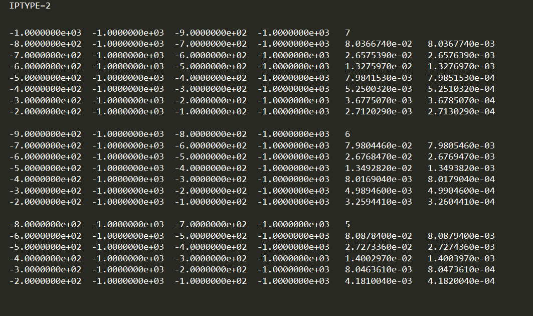
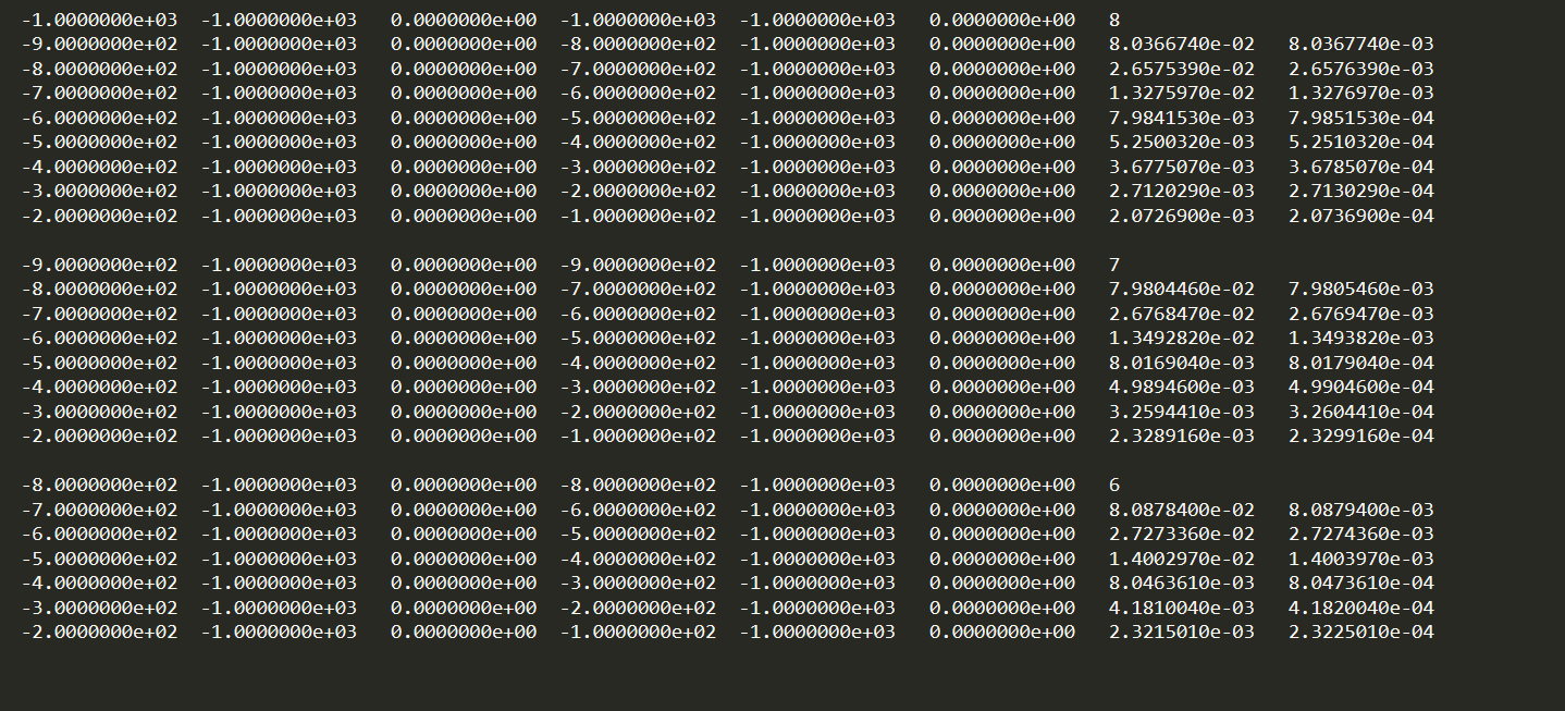
3.3.3.1. Example 1: Dipole-Dipole Surface Data

For electrodes defined only on the surface, the vertical location is determined by the topography. As a result, columns for the vertical position of each electrode are not required. Below, we see the format for DC and IP observed data files. In this case, there are two sources, each with a different number of receivers.

Observed Surface DC Data

../../_images/dobs_dipole_dipole_XY_dc.PNG

Observed Surface IP Data

../../_images/dobs_dipole_dipole_XY_ip.PNG

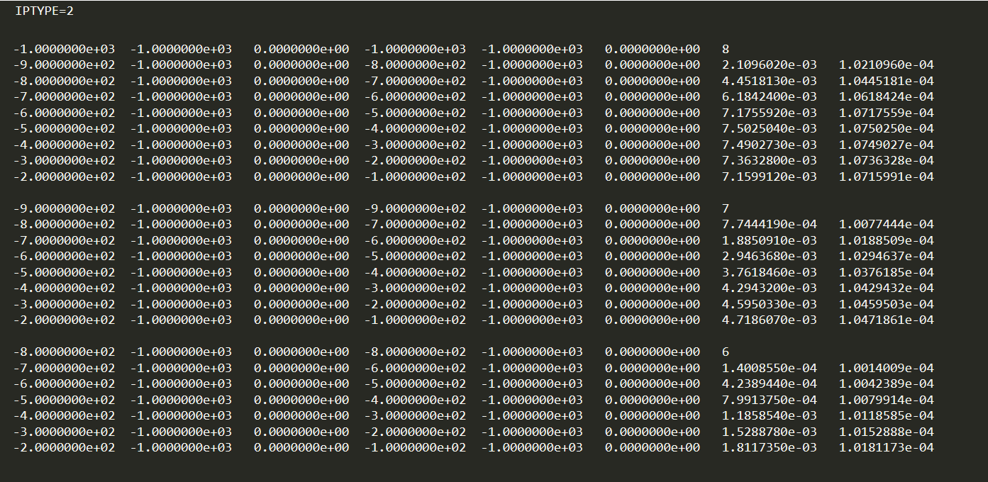
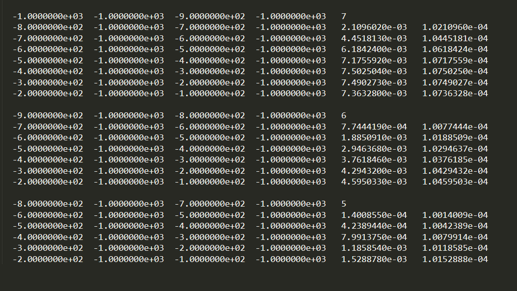
3.3.3.2. Example 2: Pole-Dipole Data with General Format

For the general data format (surface and/or borehole), the vertical locations of the electrodes are defined. Below, we see the format for DC and IP observed data files. Since the sources are pole sources, we see that the locations of the A and B electrodes are identical. If the receivers were poles, the M and N locations of corresponding M and N electrodes would be identical.

General Format Observed DC Data

../../_images/dobs_pole_dipole_XYZ_dc.PNG

General Format Observed IP Data

../../_images/dobs_pole_dipole_XYZ_ip.PNG