3.2.5. Sensitivity Weights
Creating sensitivity weights is a 2-step process. The user must use the executable dcsensitivity.exe to approximate the RMS sensitivities of the problem, then use sens2weights.exe to create the sensitivity weights file.
3.2.5.1. Approximating Sensitivities
The parameters used to approximate the sensitivities are defined in the following input file. The lines within the input file are as follows:
Line # |
Parameter |
Description |
|---|---|---|
1 |
path to octree mesh |
|
2 |
DC or IP survey file (locations of observations) |
|
3 |
path to conductivity model |
|
4 |
path to active cells model |
|
5 |
number of iterations used to approximate sensitivities |
|
6 |
approximation method for sensitivity computation |
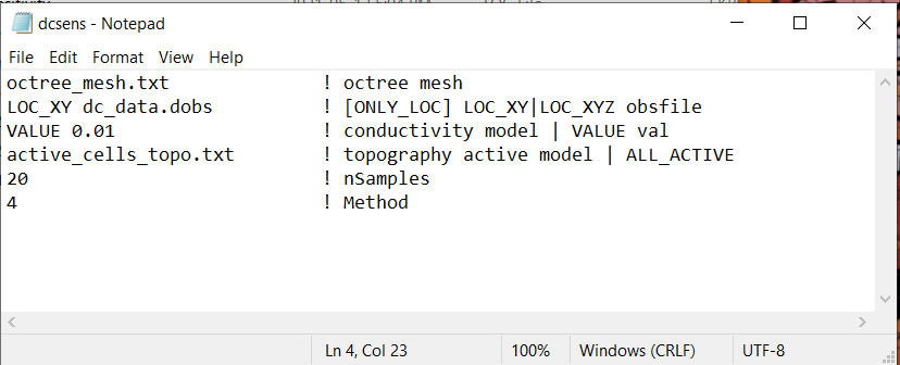
Fig. 3.5 Example input file for computing sensitivities ( Download ).
3.2.5.2. Line Descriptions
OcTree Mesh: file path to the OcTree mesh file
Survey File: This line defines the survey file. The general syntax is LOC_XY|LOC_XYZ filepath.
LOC_XY|LOC_XYZ: For surface formatted files, use the flag LOC_XY and the program will project the electrode locations to the discrete surface topography. For general formatted file, use the flag LOC_XYZ.
filepath: This is the filepath to the survey/observations file. If the file is DC data format, you will compute sensitivities for the DC inversion. If the file is IP format, you will compute sensitivities for the IP inversion.
Conductivity Model: On this line we specify the conductivity model for the sensitivity computation. On this line, there are 2 possible options:
Enter the path to a conductivity model (either starting model for DC inversion or background conductivity for IP inversion)
If a homogeneous conductivity value is being used, enter “VALUE” followed by a space and a numerical value; example “VALUE 0.01”.
Active Topography Cells: Here, the user can choose to specify the cells which lie below the surface topography. To do this, the user may supply the file path to an active cells model file or type “ALL_ACTIVE”. The active cells model has values 1 for cells lying below the surface topography and values 0 for cells lying above.
# Samples: This is the number of samples used to approximate the sensitivities. Somewhere between 5 and 20 samples are generally needed. A reasonable default value is 10. For more, see theory section . Ignored if the method for computing sensitivities is an analytic method .
Method: The method for approximating the average or root mean squared sensitivities. The user enters an integer from 1 to 5:
RMS sensitivities approximated using Hutchinson approach (\(v = \pm 1\))
RMS sensitivities approximated using Hutchinson approach (\(-1 < v < 1\))
RMS sensitivities approximated using Probing method
Analytic average sensitivities
Analytic RMS sensitivities
Note
Sensitivities computed analytically are much better for creating sensitivity weights. For reasonably sized problems, the time required to compute analytic sensitivities is comparable to the time required for any of the approximate methods.
3.2.5.3. Sensitivities to Weights
The parameters used to create a weights file from approximate sensitivities are defined in the input file below. The lines within the input file are as follows:
Line # |
Parameter |
Description |
|---|---|---|
1 |
path to octree mesh |
|
2 |
path to approximate sensitivities |
|
3 |
path to active cells model |
|
4 |
truncation factor |
|
5 |
smoothing factor |
|
6 |
output file name for sensitivity weights |

Fig. 3.6 Example input file for computing sensitivity weights model ( Download ).
3.2.5.4. Line Descriptions
OcTree Mesh: file path to the OcTree mesh file
Sensitivities: file path to the approximate sensitivities output by dcsensitivity.exe
Active Topography Cells: Here, the user can choose to specify the cells which lie below the surface topography. To do this, the user may supply the file path to an active cells model file or type “ALL_ACTIVE”. The active cells model has values 1 for cells lying below the surface topography and values 0 for cells lying above.
Truncation Factor: The dynamic range of the approximate sensitivities is very large (many orders of magnitude). But we are only interested in ensuring we do not cluster anomalous cells immediately near the electrodes. Thus we introduce a truncation factor for the weights; a value between 0.01 and 0.1 is good. The truncation factor defines the ratio between the largest and smallest weight value. And since the weights file is normalized so that a value of 1 is assigned to all unweighted cells:
Smoothing Factor: The distribution of sensitivities is very rough when approximated with Hutchinson’s or the probing methods, and may introduce artifacts in the inversion. To counteract this, the user may apply a smoothing filter. The smoothing factor is an integer value and denotes how many times the smoothing is applied. A value between 1-4 seems to work best when Hutchinson’s or probing methods were used to approximate the sensitivities. If the analytic average or RMS sensitivities were computed, this can be set to 0 or 1 .
Output Name: The output file name for the sensitivity weights file